Active learning chooses which items to label next, and the promise is the same accuracy for fewer labels. Re-evaluations under controlled conditions found the gain is real in some settings, small or absent in others, and negative when labels are very few. The savings you will get depend on your training recipe as much as on the query strategy.
The loop, and the families of query strategy
Pool-based active learning, the form Settles's 2009 survey made standard, runs a loop. Label a seed set, train a model, score the unlabelled pool, send the highest-scoring batch to annotators, retrain, repeat. Everything interesting is in the scoring rule.
Uncertainty methods pick items the current model is least sure about: lowest top-class probability, smallest margin between the top two classes, or highest entropy. Diversity methods pick items that cover the pool, as in core-set selection, which chooses points so that every unlabelled item is close to a labelled one. Hybrid methods combine both; BADGE picks a batch that is both uncertain and diverse in gradient space, which matters when batches are large. A fourth idea, typicality, picks the most representative items and comes back in the cold-start section below.
| Family | Picks | Examples | Typical weakness |
|---|---|---|---|
| Uncertainty | items the model is unsure of | least confidence, margin, entropy | redundant batches; unreliable with few labels |
| Diversity | items that cover the pool | core-set | ignores the decision boundary |
| Hybrid | uncertain and diverse | BADGE | compute cost on large pools |
| Typicality | dense, representative items | TypiClust | stops helping as budget grows |
The claimed savings versus the reproduced ones
Papers proposing a new strategy usually report a clear gain over random sampling. The papers that re-ran many strategies under one protocol report something less tidy.
Munjal et al. (2022) compared uncertainty, diversity and committee methods under identical settings and found an inconsistent gain over random sampling, with enough variance between runs to contradict previously reported results. Under strong regularisation, the methods showed marginal or no advantage over random.
Beck et al. (2021) re-implemented the main methods for image classification and reached a more positive result: with data augmentation, active learning was 2 to 4 times more label-efficient than random sampling. But once augmentation was included, BADGE no longer beat plain uncertainty sampling consistently, so much of the difference between the sophisticated methods disappeared.
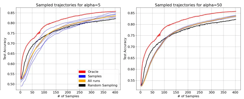
Lüth et al. (2023) traced the contradictions to five evaluation pitfalls: too few data settings, starting budgets and query sizes tested, a neglected classifier configuration, and ignored alternatives such as self-supervised pretraining. Tuning the classifier properly let their random baseline exceed the originally reported performance of several recent methods on CIFAR-10 and CIFAR-100. Werner et al. (2024) added a seed problem: with the usual three runs, which method looks best can change with the random seed, so their benchmark uses 50.
Why random sampling is a hard baseline
A random sample has two properties that a selected one lacks. It matches the distribution you will deploy on, and it is not tied to any one model. Better training recipes lean on both.
Augmentation, regularisation and self-supervised pretraining all make a model learn more from each label, and they help a random sample as much as a selected one, much as cleaner labels do in the quality-versus-quantity evidence. Lüth et al. found that combining active learning with self-supervised pretraining improved performance considerably, but that pretrained and semi-supervised models received a smaller gain from active learning over random querying than standard training did. The better your recipe, the less there is for selection to add.
The baseline does not always win. Werner et al.'s cross-domain benchmark ranked random sampling poorly on most of its text and tabular datasets and last on FashionMNIST, and noted that the image domain behaved differently from the other two. And Lüth et al. found that active learning generally brought substantial gains when classes were imbalanced, which is the common case in real annotation projects. The honest summary is that the gain is an empirical quantity for your data and recipe, and the way to find it is to measure it.
Cold start: why uncertainty fails with few labels
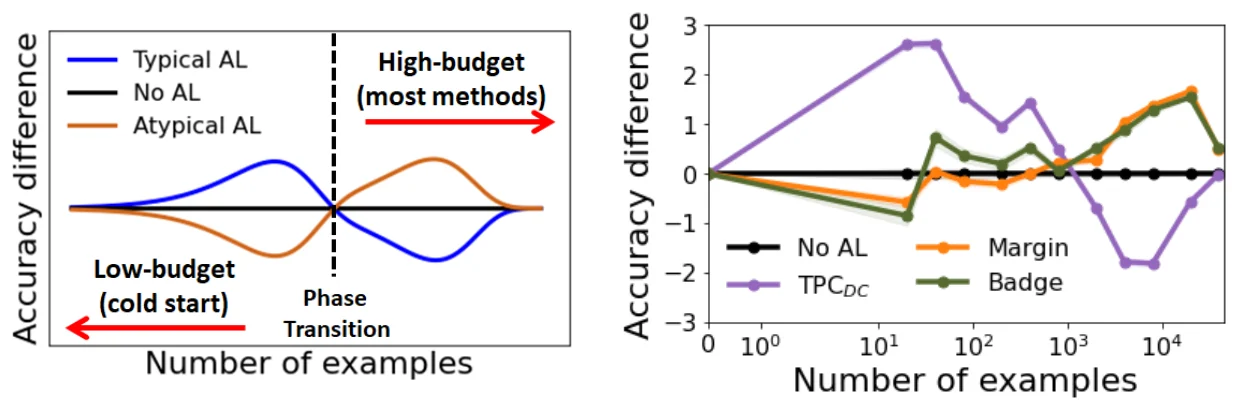
Uncertainty needs a model that knows enough to be usefully uncertain. With a handful of labels per class it does not, and its least-confident items are mostly noise and outliers.
Hacohen, Dekel and Weinshall (2022) showed the effect is a reversal, not just a weakening. With low budgets, typical examples are the best ones to label; with high budgets, the unrepresentative ones are. In their low-budget experiments, labelling 1 to 10 examples per class per round, the other active learning baselines performed on par with random selection or worse. Their typicality-based method, TypiClust, selected 10 CIFAR-10 images that let a semi-supervised model reach 93.2% accuracy, an improvement the authors put at 39.4% over random selection.
Lüth et al. located the failures of the standard methods in the same few-label settings, while finding BADGE the most reliable overall, even there.
So how many labels do you need before starting? No paper gives a universal number, but the evidence suggests a sequence. Pick the seed set for coverage rather than uncertainty, from clusters of self-supervised features or simply at random and stratified by any metadata you have. Switch to an uncertainty or hybrid method once the model is clearly better than chance on every class you care about, and keep checking that it still beats a random batch.
Sampling bias and the model-transfer problem
An actively selected training set is, by design, not a sample of your data. It over-represents the hard cases near the current model's decision boundary and under-represents the easy bulk. That is the point, and it has two consequences.
First, never evaluate on actively selected items. The test set must be a random sample, labelled separately, or the metric describes the hard cases rather than deployment. Our golden evaluation set post covers how to build one that stays clean.
Second, the selected set is tuned to the model that selected it. Lowell, Lipton and Wallace (2019) found that the benefits of active learning did not generalise reliably across models and tasks, and that training a successor model on an actively acquired dataset did not consistently outperform training it on an i.i.d. sample. Labels outlive models: the set you buy this year will train next year's architecture, and what was selected for the old one may suit the new one no better than a random draw would.
A cheap guard against both is to make a fixed share of every batch, say a fifth, a plain random draw from the pool. It grows a random sample alongside the selected one, gives you a running comparison between the two, and limits how far the training distribution drifts.
import numpy as np
rng = np.random.default_rng(0)
probs = model.predict_proba(X_pool)        # (n_pool, n_classes)
top2 = np.sort(probs, axis=1)[:, -2:]
margin = top2[:, 1] - top2[:, 0]          # small margin = uncertain

batch, random_share = 2000, 0.2
n_rand = int(batch * random_share)
rand_idx = rng.choice(len(X_pool), n_rand, replace=False)
rest = np.setdiff1d(np.arange(len(X_pool)), rand_idx)
unc_idx = rest[np.argsort(margin[rest])[:batch - n_rand]]

# send both to annotators as one shuffled batch, unmarked;
# keep the arm in your own records to compare learning curves later
When it pays, and how to run it with a vendor
Papers usually query small batches and retrain after each one. An annotation vendor works in batches with a turnaround of days and a fixed cost to set each one up, so in practice the query size is hundreds or thousands of items and the number of rounds is small. Lüth et al. list query size as one of the settings an evaluation must vary, and it is one you should agree with the vendor before the first round.
Large batches change which methods work. Plain uncertainty sampling fills a big batch with near-duplicates from the same confusing region; batch-aware methods such as BADGE, or uncertainty followed by clustering and one pick per cluster, exist for that reason.
Expect selected items to cost more per label than random ones, because they are the hard cases. The SAM data engine shows the same pattern from the other side: once the model took the easy masks, time per remaining mask went back up from 14 to 34 seconds, as described in model-assisted labelling. Price active batches by time where you can, not only by item count.
And check that the conditions for a gain actually hold:
- The unlabelled pool is large compared with the labelling budget, so there is something to choose between.
- Labels are expensive, such as expert medical, legal or engineering judgements, so every label saved repays the engineering.
- Classes are imbalanced and the rare ones matter; selection finds them faster than random draws do.
- The model architecture is stable, so the selected set will not be inherited by a very different successor.
- You can retrain between batches in less time than a batch takes to label.
Questions people ask
How does active learning reduce labelling cost?
By labelling the items that teach the model most and skipping ones it already handles, so the same accuracy is reached with fewer labels. Controlled re-evaluations put the gain anywhere from 2 to 4 times label efficiency in one image-classification study to marginal or none in others, depending on the training recipe, the budget and the data. Measure it against a random arm.
What is uncertainty sampling?
The most common query strategy: send for labelling the items the current model is least sure about. Least confidence takes the lowest top-class probability, margin sampling the smallest gap between the top two classes, and entropy the most spread-out prediction. It works once the model is reasonably trained and fails with very few labels, when its uncertainty is mostly noise.
Is active learning better than random sampling?
Sometimes. Munjal et al. found inconsistent gains and, under strong regularisation, marginal or none; Beck et al. found 2 to 4 times better label efficiency with augmentation; Werner et al. ranked random low on most text and tabular tasks. A well-tuned, pretrained model narrows the gap. Only a comparison on your own data, with several seeds, settles it.
When should you not use active learning?
When labels are cheap enough that labelling more at random costs less than the engineering, when you have only a few labels per class and would rely on uncertainty sampling, when the model will change substantially before the labels are used, or when the batch turnaround is too slow to retrain between rounds. In those cases a stratified random sample is simpler and often as good.
How many samples do you need to start active learning?
No universal number exists. Below roughly ten labels per class, the cold-start studies found uncertainty-based methods no better than random, and often worse. Start with a seed chosen for coverage, by clustering self-supervised features or by stratified random sampling, and switch to uncertainty or BADGE once the model is clearly better than chance on every class.