There is no single number, but there is a reliable method. The folklore figure of 1,000 images per class comes from ImageNet and describes training from scratch; with a pretrained backbone the floor is far lower, and each further point of accuracy costs more images than the last. The answer for your task comes from a learning curve fitted on three or four subsets of your own data.
Where the 1,000-per-class rule came from
The number most people quote traces to Pete Warden's 2017 post, which gives the rule of thumb as 1,000 representative images for each class and says plainly where it came from: the original ImageNet classification challenge. ILSVRC-2012 has 1,000 classes and about 1.28 million training images, between 732 and 1,300 per class, and it was enough to train AlexNet and its successors from random initialisation.
So the rule describes a specific situation: training a network from scratch to separate a thousand fine-grained classes. Hestness et al. (2017) trained ResNets from scratch on ImageNet subsets from 1 to 800 images per class and found that below roughly 25 images per class the error was about that of random guessing. In that setting, a few hundred per class is the bottom of the useful range and a thousand is reasonable.
The same post notes that transfer learning changes this, and that a model already trained on a similar domain can learn new classes from as few as ten or twenty examples. That caveat is the more useful half of the advice, and it is the situation most projects are now in.
Pretrained backbones moved the floor
Large pretrained models have made the few-shot end of the range respectable. Big Transfer (BiT) reports 76.8% top-1 accuracy on ILSVRC-2012 with 10 labelled examples per class, and 97.0% on CIFAR-10 with 10 per class. ViT-G/14 reaches 84.86% top-1 on ImageNet with 10 examples per class. The VTAB benchmark was built around the same premise: each of its 19 tasks gives the model 1,000 training examples in total, whatever the number of classes.
Two qualifications keep these numbers honest. The backbones were pretrained on JFT-300M and its three-billion-image successor, labelled images much like the test images in kind; the further your images are from photographs of everyday scenes, the less of that advantage carries over. VTAB splits its tasks into natural, specialised and structured groups and reports each separately; check which group your images resemble. And these are classification results; detection and segmentation ask more of every image.
A smaller medical study shows the whole curve. Cho et al. (2015) trained a classifier for six CT body-part classes on 5, 10, 20, 50, 100 and 200 images per class. Mean accuracy rose from 8.01% at 5 per class to 51.54% at 20, 89.68% at 100 and 95.67% at 200.
| Setting | Labelled images | Result | Source |
|---|---|---|---|
| ImageNet, from scratch | under ≈25 per class | near random guessing | Hestness et al. 2017 |
| ImageNet, BiT-L transfer | 10 per class | 76.8% top-1 | Kolesnikov et al. 2020 |
| ImageNet, ViT-G/14 transfer | 10 per class | 84.86% top-1 | Zhai et al. 2022 |
| CIFAR-10, BiT-L transfer | 10 per class | 97.0% | Kolesnikov et al. 2020 |
| CT body parts, 6 classes | 200 per class | 95.67% mean | Cho et al. 2015 |
What learning curves show about diminishing returns
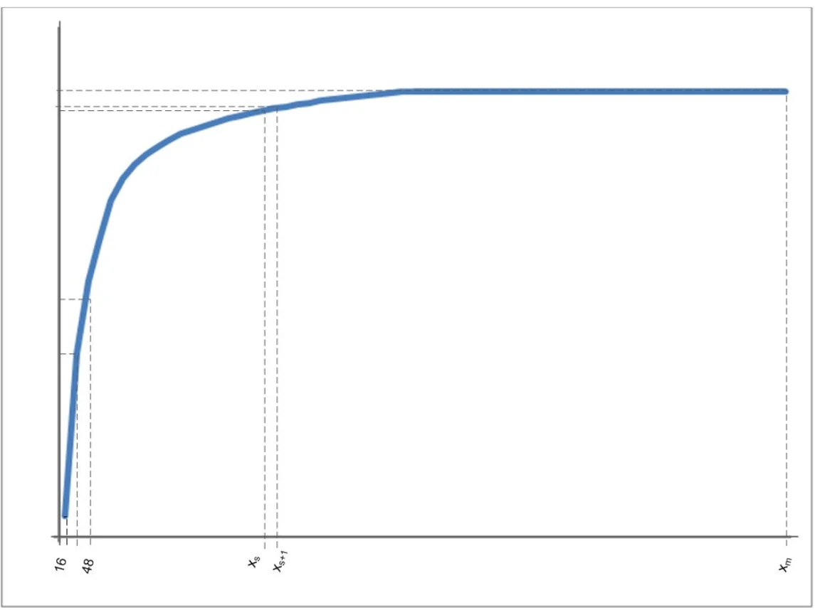
The shape of the curve matters more than any single point on it. Sun et al. (2017) trained on subsets of JFT-300M, 300 million images with more than 375 million noisy labels, and found that performance on vision tasks increases logarithmically with the volume of training data: each tenfold increase buys roughly the same improvement as the last one did.
Hestness et al. describe the same thing as a power law with three regions: a small-data region where the model is barely better than guessing, a power-law region where error falls steadily, and an irreducible-error region where more data stops helping. For ImageNet top-1 error they measured an exponent of −0.309, and for top-5 error −0.488. The arithmetic matters for budgets: with an exponent of 0.309, halving the error takes about 9.4 times the data; with 0.488, about 4.1 times.
Cho et al. show what this means for a budget. Their fitted curve predicted that the CT classifier needed 4,092 images per class to reach 99.5% accuracy, against 200 per class for 95.67%. The curve also predicted 98% at 1,000 per class, and the measured result was 97.25%, close enough to plan with.
Label quality moves the whole curve, not just one point on it: noisy labels raise the floor that more data approaches. Our post on quality versus quantity collects the evidence on that trade.
Instances, not images: detection and segmentation
For detection, the unit of supervision is the labelled object. COCO has about 2.5 million labelled instances in 328,000 images, and its paper reports 7.7 instances per image on average, so an image count says little about how much a detector is learning. Our YOLO training post gives Ultralytics' best-results guidance in instances per class and what a workable starting point looks like.
Instances in the same image are not independent, though. Twelve pallets in one photograph share the lighting, the camera, the background and usually the distance, so they teach less than twelve pallets photographed in twelve places. The effective sample size sits between the image count and the instance count, closer to the images when scenes repeat. Count both, and count distinct scenes or sites as a third number.
Segmentation supervises every pixel, so each image carries more signal and datasets tend to be smaller in image count. The finely annotated training split of Cityscapes has 2,975 images. The Medical Segmentation Decathlon chose its heart task, 30 MRI scans in total, for its combination of a small training set and large anatomical variability. For semantic segmentation the binding count is often pixels of the rare classes: poles, signs and thin structures occupy a sliver of each image, and their boundaries are where models fail.
- Classification: count images per class, and distinct sources per class.
- Detection: count instances per class, images containing each class, and the spread of object sizes.
- Segmentation: count masks or annotated pixels per class, and images in which each rare class appears.
The rarest class sets the budget
Aggregate accuracy averages over classes, and the common ones dominate it. A dataset with 5,000 images of one class and 80 of another has an 80-image problem. LVIS, built for exactly this long tail, labels each category rare if it appears in 1 to 10 training images, common for 11 to 100 and frequent above 100, and reports average precision separately for each group, so that the tail is not hidden by the head.
So size the order per class. Read off, for each class, how many examples its own learning curve says it needs, and let the hardest class that matters set the total. That class is usually the rarest, but not always: in Cho et al. every class had the same number of images, yet at 200 per class accuracy ranged from 88.45% for the pelvis to 99.61% for the chest.
There are four ways out when a rare class is too expensive to collect at random: target its collection directly, merge it with a neighbour if the application allows, handle it in a second-stage model, or supplement it with generated images, whose limits our synthetic data post sets out. Finding rare items in a large unlabelled pool is also where the evidence for active learning for annotation is most encouraging.
Fit your own curve, then turn it into an order
The forecast that holds up is one fitted on your own data. Figueroa et al. (2012) fitted inverse power-law learning curves with a weighted least-squares method and found that, depending on the dataset and sampling method, 80 to 560 labelled samples were enough for the fitted curve to predict later performance with mean absolute and root-mean-square errors below 0.01. Their tasks were text and signal classification, but the method does not care what the inputs are.
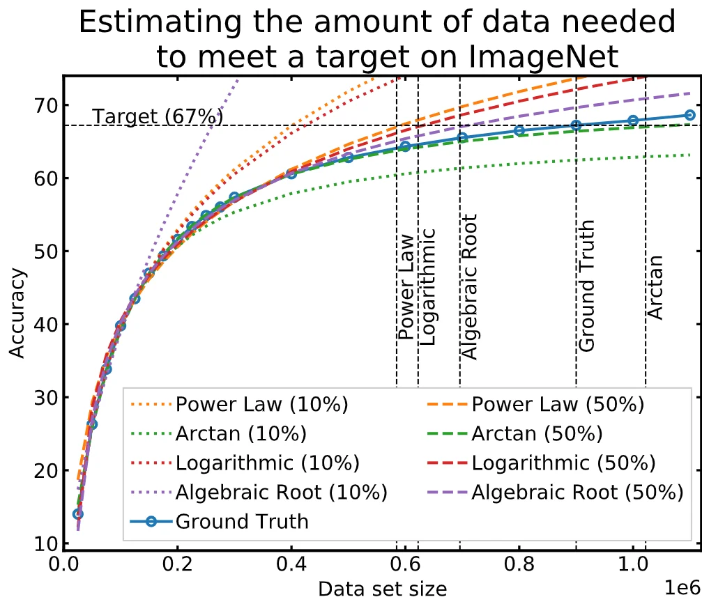
Extrapolation has a known bias. Mahmood et al. (2022) tested regression functions on classification, detection and segmentation and found that power-law, logarithmic and algebraic-root fits tend to under-estimate how much data is needed, while an arctan fit tends to over-estimate, by up to five times on CIFAR-100, ImageNet and VOC. On ImageNet, curves fitted on 600,000 images came within 1% to 6% of the true accuracy and still misjudged the data needed for a 67% target by 120,000 to 310,000 images. Their advice is to collect in up to five rounds and to correct an optimistic fit rather than trust it once.
Turning the forecast into an order is then arithmetic: the per-class need for the hardest class that matters, times the number of classes, plus a separate random test set that never enters the curve, bought in rounds with a refit after each. The free fine-tuning data calculator gives pilot, workable and strong sizes by task as a first guess before you have a curve of your own.
- Label a stratified pilot set and a separate test set; the test set stays fixed throughout.
- Train on nested subsets, for example 12.5%, 25%, 50% and 100% of the pilot, with three seeds each, and record the validation metric per class.
- Fit error = a·n−b + c per class, where c is the floor more data approaches.
- Read off the n that reaches your target for the hardest class that matters; treat it as a lower bound.
- Order the next round, retrain, refit, and stop when the curve, not the plan, says the target is reached.
import numpy as np
from scipy.optimize import curve_fit

n   = np.array([250, 500, 1000, 2000])      # images per class in each subset
err = np.array([0.31, 0.24, 0.19, 0.155])   # validation error, mean of 3 seeds

def curve(n, a, b, c):                       # inverse power law with a floor
    return a * n ** (-b) + c

(a, b, c), _ = curve_fit(curve, n, err, p0=[1.0, 0.5, 0.05],
                         bounds=([0, 0, 0], [np.inf, 2, 1]))
target = 0.12
need = ((target - c) / a) ** (-1 / b) if target > c else float("inf")
print(f"floor {c:.3f}, exponent {b:.2f}, ~{need:,.0f} per class for {target:.0%} error")
# floor 0.069, exponent 0.50, ~5,740 per class for 12% errorQuestions people ask
How many images do you need to train a CNN?
From scratch, hundreds to about a thousand per class: on ImageNet, ResNets trained on fewer than roughly 25 images per class did little better than chance. Fine-tuning a pretrained backbone needs far fewer, often tens to a few hundred per class for distinct classes. The reliable answer comes from training on a few subset sizes of your data and fitting the learning curve.
Is 100 images enough to train a model?
Sometimes, if it means 100 per class, a pretrained backbone and visually distinct classes. Large pretrained models reach 77% to 85% ImageNet accuracy from 10 per class. A hundred images in total across several classes is a pilot rather than a training set: enough to fit the first point of a learning curve and see how steep it is.
How many images per class for image classification?
With transfer learning, a few hundred per class is a reasonable pilot and often enough; the 1,000-per-class rule describes training from scratch on ImageNet. In one medical study, 200 per class gave 95.67% mean accuracy and the fitted curve put 99.5% at 4,092 per class. Let the hardest class that matters, measured on its own curve, set the number.
Do more instances per image count as more data?
Partly. A detector learns from each labelled object, so instances are the main unit for detection, and COCO averages 7.7 per image. But instances in one image share lighting, camera and background, so twelve objects in one scene teach less than twelve objects in twelve scenes. Track images, instances and distinct scenes per class.
How many images do I need for object detection?
Think in instances per class and in the range of conditions they cover. Ultralytics' guidance for best results is 1,500 images and 10,000 instances per class, and a few hundred instances of a distinct class can give a workable detector from pretrained weights. Fit a learning curve on your own subsets to see where between those your classes sit.