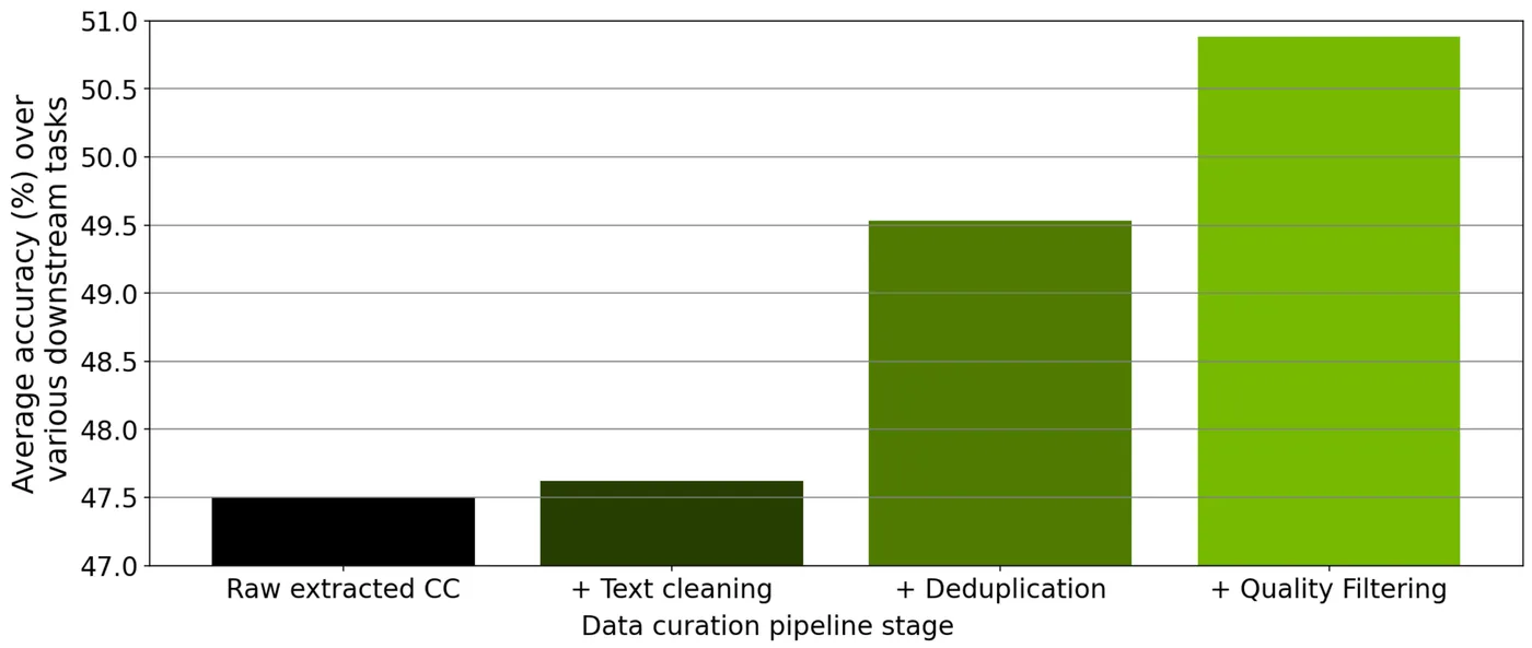
Deduplication is the highest-value-per-hour operation in data preparation. It costs compute rather than judgement, every major corpus does it, and skipping it silently inflates your benchmark scores.
Three kinds of duplicate, three different harms
Worth separating, because they need different detection and cause different problems.

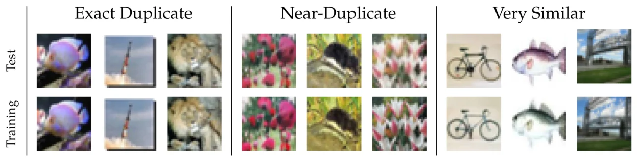
Exact duplicates. Byte-identical records. Simple to detect, trivially cheap, and common in anything assembled from multiple sources. They waste compute and overweight whatever they contain.
Near duplicates. The same content with minor differences — a reformatted document, a re-uploaded image, boilerplate with one field changed, the same article on two sites. These are the bulk of real duplication and need fuzzy matching to find.
Cross-split duplicates. The same or near-same item in both training and evaluation. This is the one that actually damages you, because it inflates your metrics. Your model has seen the test answers and your evaluation is measuring memorisation. Every benchmark number you report is then wrong in the flattering direction.
What the big corpora did
The published pipelines give you tested defaults rather than guesses.
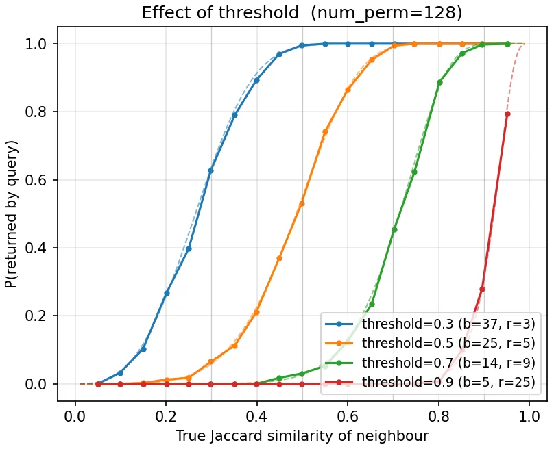
FineWeb used MinHash with 5-gram shingles and 112 hash functions, arranged as 14 buckets of 8 hashes, targeting roughly 75% similarity — and applied it per crawl dump independently rather than globally, which is an unusual choice worth noting if you are copying the recipe.
RedPajama-Data-v2 flagged exact duplicates with a Bloom filter over content hashes, and ships MinHash signatures computed with 128 hash functions so that you can add fuzzy matching at the similarity level you choose. By the figures in its paper, dropping those exact duplicates takes the head and middle partitions from 32.8 billion documents and 50.7 trillion tokens to 20.8 billion and 30.4 trillion — roughly 40% of the tokens removed.
That 40% figure is the one to carry around. Web-derived data is massively redundant, and if your pipeline is not removing a substantial fraction you should check whether it is working at all.
import hashlib, re
from datasketch import MinHash, MinHashLSH

def norm(t):                                  # normalise before hashing
    return re.sub(r"\s+", " ", t.strip().lower())

def shingles(t, k=5):
    w = norm(t).split()
    return {" ".join(w[i:i+k]) for i in range(max(1, len(w) - k + 1))}

# 1. exact - cheap, do it first, it shrinks the problem
seen, rows = set(), []
for r in corpus:
    h = hashlib.sha256(norm(r["text"]).encode()).hexdigest()
    if h not in seen:
        seen.add(h); rows.append(r)
print(f"exact: {len(corpus)} -> {len(rows)}")

# 2. near-duplicates via MinHash LSH
lsh, kept = MinHashLSH(threshold=0.75, num_perm=128), []
for i, r in enumerate(rows):
    m = MinHash(num_perm=128)
    for s in shingles(r["text"]):
        m.update(s.encode())
    if not lsh.query(m):                      # nothing similar already kept
        lsh.insert(str(i), m); kept.append(r)
print(f"near: {len(rows)} -> {len(kept)}")

# 3. cross-split - the one that matters. Always TRAIN side loses.
eval_lsh = MinHashLSH(threshold=0.70, num_perm=128)
for j, e in enumerate(eval_set):
    m = MinHash(num_perm=128)
    for s in shingles(e["text"]):
        m.update(s.encode())
    eval_lsh.insert(f"e{j}", m)

clean, leaked = [], 0
for r in kept:
    m = MinHash(num_perm=128)
    for s in shingles(r["text"]):
        m.update(s.encode())
    if eval_lsh.query(m):
        leaked += 1                           # drop from TRAIN, keep eval intact
    else:
        clean.append(r)
print(f"cross-split leaks removed from train: {leaked}")Choosing a threshold
Similarity thresholds are a judgement call and the consequences are asymmetric, which should guide you.
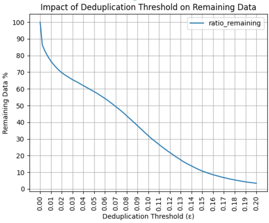
Too aggressive and you discard legitimately distinct items that happen to share structure — a real risk with templated text, short records, or code, where boilerplate dominates the token overlap. Too lenient and near-duplicates survive.
The published corpora cluster around 0.70 to 0.80 for text, which is a reasonable starting range. For cross-split checking, bias lower — be more aggressive — because a false positive costs you one training example and a false negative costs you the integrity of your evaluation.
Inspect the pairs your threshold catches. Print twenty pairs at the boundary and decide whether you would call them duplicates. Ten minutes calibrates the threshold far better than reasoning about it, and it is the step that catches a badly wrong setting before it removes half your data.
Images, audio and code need different methods
Text shingling does not transfer, and each modality has a standard approach.
Images. Perceptual hashing catches resizes, recompressions and minor crops cheaply. Embedding similarity catches semantic near-duplicates — the same scene from a slightly different angle — which perceptual hashing misses and which matters for cross-split leakage. Video frames are the acute case: consecutive frames are near-identical, so a random split over frames guarantees leakage, and you must split by clip.
Audio. Audio fingerprinting for exact and near matches. The same trap as video applies: split by recording or speaker, never by segment.
Code. Exact and token-level matching after normalising whitespace and comments. Code is extraordinarily duplicated — vendored dependencies, forks, generated files, the same snippet copied across thousands of repositories. Expect to remove a lot, and consider excluding obviously generated and vendored paths before you start.
Keep the counts
Log how many records each deduplication stage removed, and keep that with the dataset's provenance record — see our provenance post.
Two reasons. It is how you notice that a pipeline change silently stopped working, which happens and is otherwise invisible. And it is how you explain the composition of a mixture later, when someone asks why the model over-weights a particular source.
The counts also tell you something about your sources. A source that loses 90% to deduplication was mostly repetition, which is useful information about whether to include it next time.
Questions people ask
Should I deduplicate before or after filtering?
Exact deduplication first, because it is cheap and shrinks everything downstream. Quality filtering next. Near-duplicate detection after that, since it is the expensive stage and you want it running over the smallest possible set. Cross-split checking last, immediately before training.
Does deduplication hurt if my data is naturally repetitive?
Legitimate repetition — common phrases, standard forms, boilerplate that genuinely occurs at that frequency in your domain — is signal, and aggressive deduplication can flatten it. Deduplicate at the document level rather than the passage level, and calibrate your threshold by inspecting boundary pairs.
How do I check for leakage against a benchmark I did not build?
Run the same near-duplicate check between your training data and the benchmark's public test set. If you find overlap, you cannot report that benchmark honestly without saying so — which is one of several reasons a private evaluation set is worth building.
Is deduplication enough to prevent memorisation?
It reduces it substantially, since repeated content is memorised most readily, but it does not eliminate it — models can memorise singly-occurring content, particularly distinctive strings. If memorisation is a specific concern, it needs its own testing.