Mid-training is a recent name for a stage that frontier labs had been running quietly for a while: a short, curated, high-quality run at the end of pretraining, with the learning rate decaying to zero. It is cheap and it moves benchmarks a lot.
The definition, and who gave it
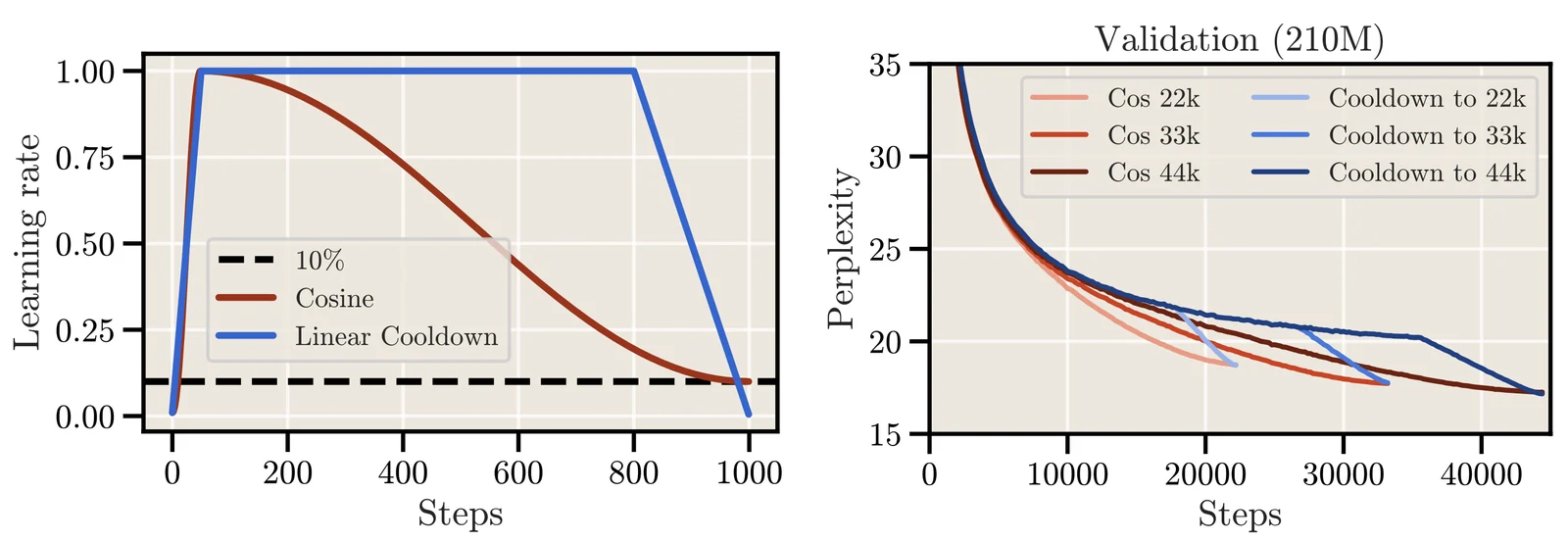
OLMo 2 supplies the clearest primary definition: “During the second stage, which we refer to as mid-training (5–10% of training FLOPs), we up-sample the highest-quality web documents and curated non-web sources”. Over that stage the learning rate is linearly decayed to zero. Its stated purpose is to “imbue the model with domain knowledge from increased exposure to STEM references and high quality text”.
The terminology is still settling — the same stage gets called annealing, the decay phase, or stage two, and there is now a dedicated survey literature on it. What is stable is the shape: short, late, curated, learning rate to zero.
It is distinct from continued pretraining mainly in when it happens. Mid-training is part of the original training run, performed by whoever pretrained the model. Continued pretraining is what you do afterwards to a finished base model. The data and mechanics are similar; the ownership differs — which matters, because mid-training is a lever you only have if you are pretraining.
The numbers
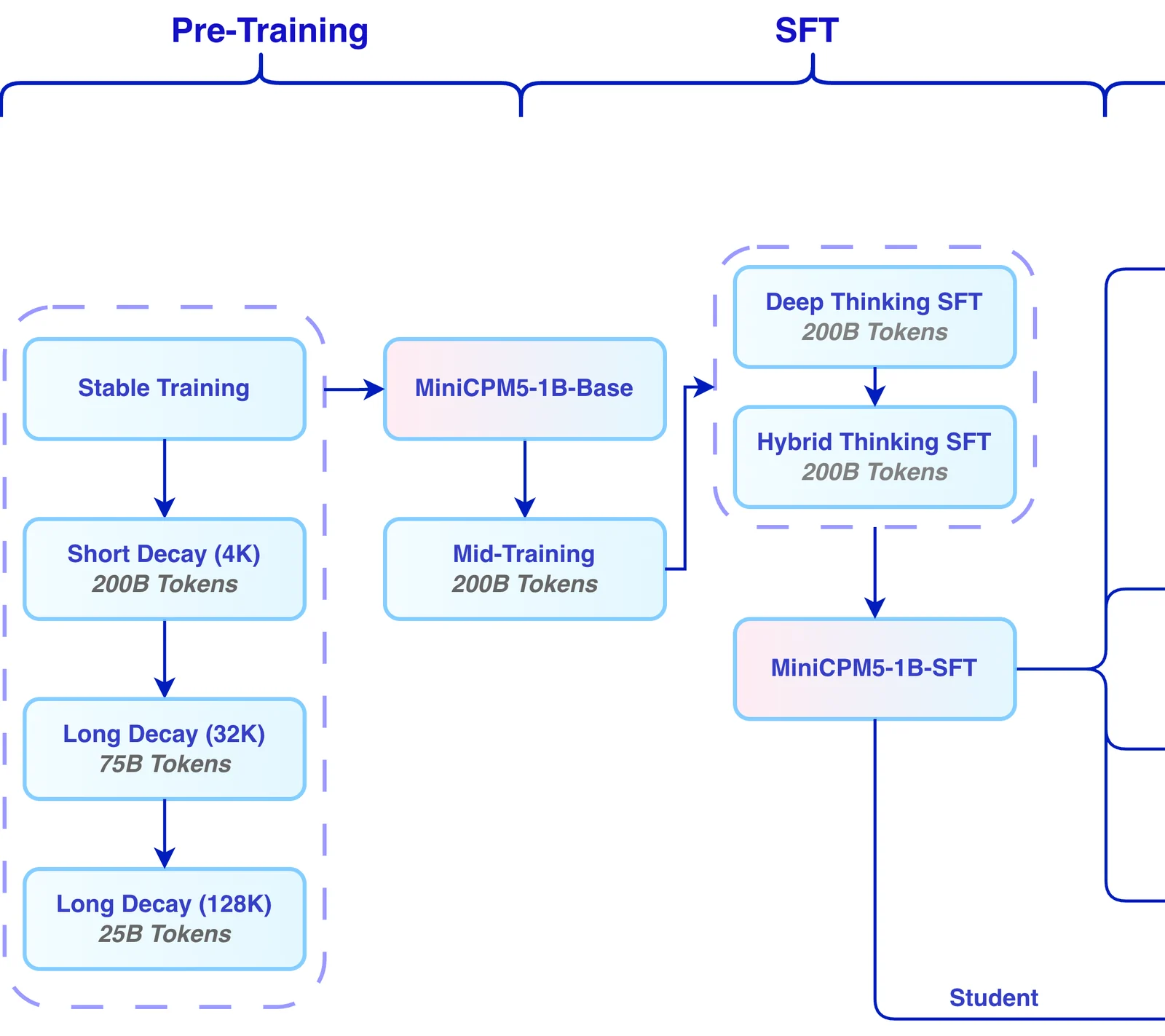
OLMo 2 publishes its structure in full. Its 7B model anneals “three separate times for 50B tokens each”; the 13B and 32B models run three passes of 100B each plus one of 300B.
The totals show how small a share this is: OLMo 2 7B is trained on 4.05 trillion tokens of which 3.90 trillion is stage-one pretraining — so roughly 150 billion tokens, under 4% and so below the 5–10% the definition gives, is mid-training. The 32B model sees 6.6 trillion total against 6.06 trillion pretraining, by the paper's rounding: its four mid-training runs (3 × 100B + 300B) make the sum 6.66 trillion.
Its curated mix, Dolmino-Mix-1124, lists a high-quality total of 832.6B tokens from which those 50B, 100B and 300B samples are drawn, alongside a separate 10.7B-token maths mix. The paper releases its artefacts under Apache 2.0 wherever possible; the dataset card itself states ODC-By.
| Model | Total tokens | Stage-one pretraining | Mid-training structure |
|---|---|---|---|
| OLMo 2 7B | 4.05T | 3.90T | 3 × 50B |
| OLMo 2 13B | 5.6T | 5.0T | 3 × 100B + 1 × 300B |
| OLMo 2 32B | 6.6T | 6.06T | 3 × 100B + 1 × 300B |
What it is worth
Llama 3 gives the clearest value measurement. Annealing with the GSM8K and MATH training sets in its mix of high-quality code and maths data improved a pretrained 8B model by 24.0% on GSM8K and 6.4% on MATH validation sets.
On the 405B model the paper found the gains negligible, but for an 8B model that is a large gain for a few percent of the compute, which is the entire reason the stage exists. The learning rate decaying to zero appears to matter: the model is being settled into a good region on good data rather than continuing to roam.
Llama 3 also notes a final detail that is easy to overlook — during pretraining on the last 40M tokens it annealed the learning rate linearly to zero. The decay is not only a mid-training device but the standard way to end a run.
Annealing as a cheap way to evaluate a dataset
The most immediately useful idea in this literature is a side effect. Llama 3 describes using annealing as a data-quality evaluation protocol: take a model trained to roughly half its budget, anneal the learning rate linearly to zero over 40B tokens with 30% weight on the candidate dataset, and measure what moves.
That is a far cheaper way to decide whether a corpus is worth including than a full training run, and the pattern transfers down in scale. If you are assembling a continued-pretraining mix, a short annealing run with your candidate data weighted in is a legitimate and affordable test of whether it helps.
It also gives you a defensible answer to “why is this dataset in the mix”, which is more than most data decisions can claim.
What goes in the mix
The published mixes share a character: this is where the good stuff goes.
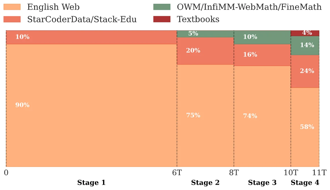
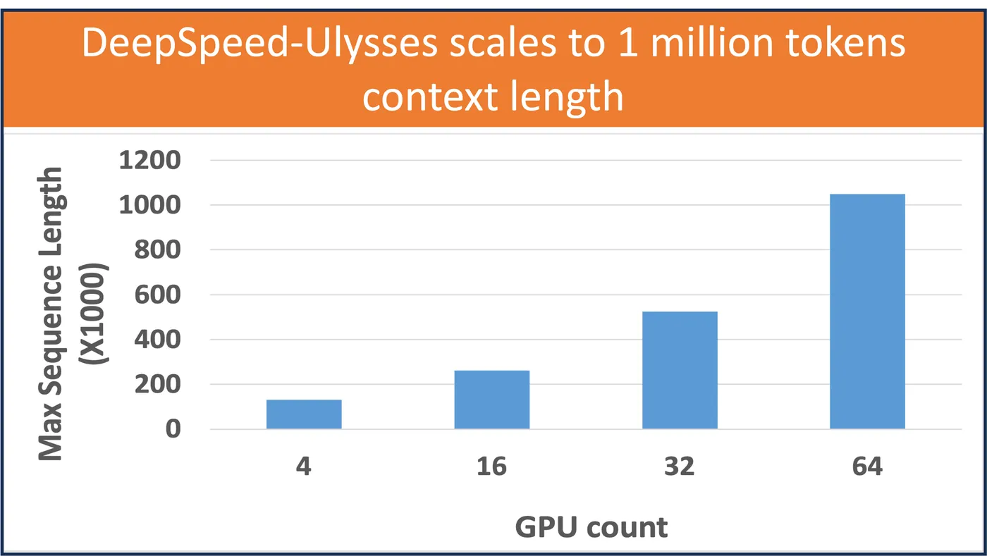
STEM references and textbook-quality explanatory text. Maths, in quantity disproportionate to its share of the web. Code. Long-context examples, where the context window is being extended — Llama 3 used approximately 800B training tokens to go from 8K to 128K in six stages. Curated encyclopedic and scientific sources.
What does not go in: the broad web crawl that made up the bulk of stage one. The point of the stage is the shift in distribution toward material the model should end up weighted towards.
If you are selecting a base model rather than training one, this is worth knowing as a reading skill. When a model card describes a two-stage or annealed pretraining run with a curated final mix, that is a signal about where its strengths will be — often maths and code, because that is what tends to get upsampled.
Questions people ask
Is mid-training the same as continued pretraining?
Mechanically similar, organisationally different. Mid-training is the final curated phase of the original pretraining run, done by whoever pretrained the model. Continued pretraining is what you do to a finished base model afterwards. If you are starting from an open base model, continued pretraining is the stage available to you.
Can I do mid-training on an open base model?
Not strictly — the stage is defined by its position in the original run, and the learning rate schedule has already completed. What you can do is continued pretraining with the same ingredients: curated high-quality domain data, a low learning rate decayed to zero, a short run, and general data mixed in to limit forgetting.
Why does annealing the learning rate to zero help?
The published results establish that it does rather than explaining why. The working intuition is that a decaying rate on high-quality data settles the model into a good region instead of continuing to move, so the final weights reflect the best data disproportionately. Treat that as a plausible account rather than a demonstrated mechanism.
How do I know whether a base model had this stage?
Read the model card and the technical report, where open models increasingly describe it explicitly — OLMo 2 names its stages and token counts. A described curated final phase heavy in maths and code is a reasonable predictor of relative strength there.