Anomaly detection exists because some problems cannot be framed as balanced classification. Understanding why reframes what data you need — and it is mostly data you already have.
An honest note on availability
Searching our verified set of 434 open datasets for sets whose documentation describes them as anomaly or outlier detection data returned only a handful — too few to make an honest list of.
That is not a gap in Dataset Finder so much as a property of the task. Anomalies are domain-specific to a degree that makes public datasets much less transferable than in other vision tasks: a surface defect on one alloy under one lighting rig looks nothing like the same nominal defect class elsewhere. So the field relies on a small number of well-known benchmarks plus everyone's own data.
Which means the useful content here is method rather than a shortlist. Our industrial inspection datasets post covers the industrial sets that do exist in Dataset Finder.
Why classification fails here
The structural property is that you cannot enumerate the positive class. A production line running well produces overwhelmingly good parts; the defects that occur are varied; and new defect types appear that were not in your training data.
A supervised classifier trained on that distribution learns the prior. It says “normal” and, on a line where 99.7% of parts are good, is right 99.7% of the time, which looks excellent and is worthless. Worse, it can only recognise defect types it has seen, and the whole point is usually to catch the ones you have not.
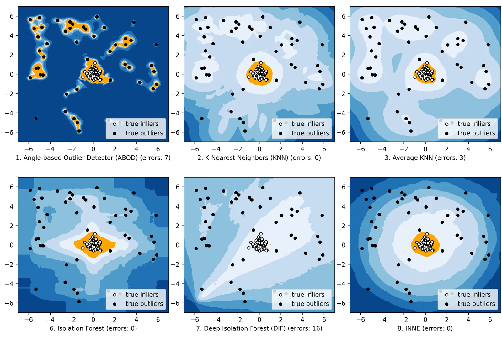
So the approach inverts: model what normal looks like, and flag deviation from it. One-class and reconstruction-based methods, density estimation, and embedding-distance approaches all share this shape. None of them need many examples of the anomaly.
What makes a good normal set
Since this is the valuable half, it is worth being deliberate about.
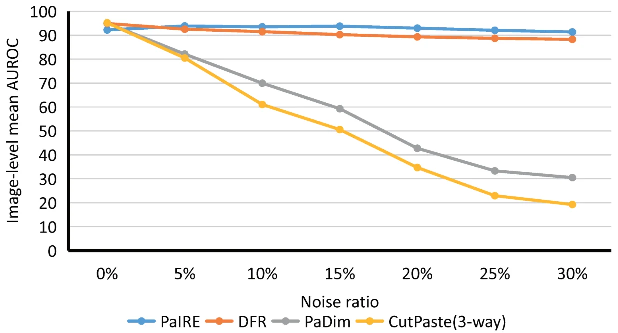
Genuinely clean. Any anomalies lurking in your normal set teach the model that those are normal, which is precisely the failure you are trying to prevent. If your normal data is “everything that passed inspection”, it contains whatever inspection missed. Worth a review pass.
Covering the full range of acceptable variation. This is where most deployments fail. Normal includes the whole legitimate range: every product variant, every lighting condition across a day and a season, every acceptable tolerance, the state of the line after maintenance and before. Anything legitimate but absent from your normal set will be flagged as an anomaly, and that is how a system ends up ignored for crying wolf.
Temporally representative. Processes drift. A normal set from one month encodes that month's conditions, and your false-positive rate will climb as reality moves away from it. Plan for periodic refresh rather than treating the model as finished.
The anomaly set is for evaluation
You still need labelled anomalies — just far fewer, and for a different purpose.
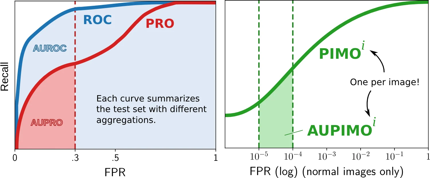
Their job is to tell you whether the method works and where to set the threshold. That means they should cover the defect types you care about, including the subtle ones, and your evaluation should report performance per defect type rather than in aggregate — a method that catches gross defects and misses hairline cracks has an excellent average and may be useless.
The honest benchmark design, and the thing to check in any public set you use: the test split should contain anomaly types absent from anything used in development. That is what tests generalisation to unseen defects, which is the actual requirement. Our golden eval set post applies directly, and this is a case where building it first genuinely changes what data you collect.
Threshold setting is a business decision rather than a technical one: the cost of a missed defect against the cost of a false alarm. Produce a curve and let the people who own those costs choose the point.
When supervised classification is right after all
Worth stating the exception, because anomaly detection is sometimes reached for unnecessarily.
If you have a small, stable, well-understood set of defect types that genuinely covers what occurs, and you can collect a few hundred examples of each, supervised classification is simpler, more accurate on those classes, and easier to explain. The anomaly framing earns its complexity when the defect set is open-ended.
A pragmatic hybrid is common and often best: an anomaly detector catches anything unusual, and a classifier labels the types you know about. The detector handles the open-ended part, the classifier handles triage, and you get both specificity and coverage.
Questions people ask
How many normal examples do I need?
Enough to cover the full range of acceptable variation, which is a coverage question rather than a count. Thousands is typical for industrial imagery, but a thousand spanning every variant and lighting condition beats ten thousand from one shift.
How many anomalies do I need?
For evaluation, enough per defect type to be meaningful — a few dozen each is a workable floor. You do not need them for training, which is the point of the approach and the reason it suits problems where defects are genuinely rare.
Can I generate synthetic defects?
Sometimes usefully, for method development and for augmenting an evaluation set. The risk is that synthetic defects are recognisably synthetic, so a detector tuned on them may miss real ones. Validate against real defects before trusting the numbers.
Does this apply outside vision?
Entirely — the same framing covers fraud detection, network intrusion, equipment telemetry and quality monitoring in any modality. The reasoning about a clean, fully representative normal set and an evaluation-only anomaly set transfers directly.